This summary covers how causality disappeared from statistics and how correlation came to dominate from the mid-19th to early 20th century, and then how causality began to attract renewed attention. It centers on the attempts by Francis Galton and Karl Pearson to emphasize correlation while excluding causality, and the story of how Sewall Wright reopened the possibility of causal inference through an innovative tool called the path diagram. Along the way, important questions are raised about the nature of statistics, the conflict between objectivity and subjectivity, and the depth of data interpretation.

1. Galton's Heredity Research and the Discovery of Regression

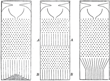
On February 9, 1877, at the Royal Institution in London, Francis Galton -- Charles Darwin's cousin and the inventor of fingerprint identification -- gave a lecture titled "The Typical Laws of Heredity." He began his talk by demonstrating a device called the Quincunx, also known as the Galton board. In this device, small metal balls dropped through a hole at the top would bounce randomly left or right off pegs as they fell, accumulating in bins at the bottom. While the path of any individual ball was unpredictable, releasing many balls always produced a remarkable regularity: a bell-shaped curve. This was a visual demonstration of the central limit theorem, proven by Pierre-Simon Laplace in 1810 -- the principle that the sum of random processes always follows a normal distribution. This law was compared to how insurance companies profit even amid uncertainty.

Galton conceived of the Quincunx as a causal model for how genetic traits like human height are inherited. But this model raised a puzzle: as the number of rows of pegs increased, the width of the bell curve should keep widening, yet the actual distribution of human height remained relatively constant across generations. He had reportedly been puzzling over this mystery for about eight years.

Galton's primary interest was not human height but human intelligence. In his 1869 book Hereditary Genius, he tried to prove that genius was inherited through family lines. He painstakingly investigated the family trees of 605 "eminent" Englishmen, but found that their sons and fathers were less eminent, and their grandparents and grandchildren even less so. While today we might point to flaws in his approach -- such as the definition of "eminence" or the influence of privilege -- at the time, he stubbornly pursued a genetic explanation.

Nevertheless, Galton made an important discovery. Studying a trait that was easy to measure and closely related to heredity -- height -- he found that tall fathers' sons were taller than average, but not as tall as their fathers. Similarly, short fathers' sons were shorter than average, but not as short as their fathers. Galton initially called this phenomenon "reversion" and later named it "regression toward mediocrity." This "regression to the mean" phenomenon appears universally in many other domains. For example, the "sophomore slump" in baseball, where Rookie of the Year winners decline the following season, is one such case.

• "Success = talent + luck. Great success = a little more talent + a lot of luck."
• "The Rookie of the Year probably had more talent than average, but also had a lot of luck. The next season, he won't be as lucky, and his batting average will drop."

Galton came to understand regression as a law of statistics rather than a law of heredity. He believed regression to the mean had some causal explanation and demonstrated a Quincunx with a ramp installed between two layers of peg arrays. This ramp funneled the balls back toward the center, keeping the bell-shaped distribution at a constant width across generations.

He reportedly said:

• "The process of reversion cooperates with the general law of deviation."

Like Hooke's law describing a spring's tendency to return to equilibrium, he inferred that regression to the mean was a physical process -- nature's way of keeping the population distribution constant.

But this thinking was mistaken. In 1877, Galton thought regression to the mean was a causal process like a law of physics, but it is merely a statistical phenomenon that often needs no causal explanation. The same is true of the sophomore slump in baseball. Experts try to find causal explanations -- players becoming complacent, opponents figuring out their weaknesses -- but in fact, it is far more often the case that it occurs simply due to the laws of probability.

2. Galton's Discovery of Correlation and Pearson's Exclusion of Causality

By 1889, as Galton gained a deeper understanding of regression to the mean, he took an important first step in separating statistics from causality. While studying "anthropometric" statistics -- collecting various body measurements such as height, forearm length, and head length -- he discovered that regression to the mean also appeared between height and forearm length. That is, tall men had longer forearms than average, but not as much longer as they were tall. Clearly, height didn't cause forearm length or vice versa. Both were likely caused by genetic factors. To describe this relationship, Galton coined the new word "co-related," later settling on the familiar term "correlated."

He made an even more surprising realization: in intergenerational comparisons, the temporal order could be reversed. In other words, if a son was taller than average, his father was also taller than average but shorter than the son. Once he realized this, Galton had no choice but to abandon any causal explanation for regression. A son's height cannot influence his father's height.

• "Wait a moment! Tall fathers usually have shorter sons, and tall sons usually have shorter fathers? How can both be true? Can a son be both taller and shorter than his father?"

The answer lies in the fact that we are dealing with two groups, not individual father-son pairs. For example, a group of fathers who are 6 feet tall are above average, so their sons will regress to the mean at an average of about 5 feet 11 inches. But the group of 6-foot father-son pairs and the group of 5-foot-11-inch son-father pairs are different. The latter group would include a few fathers taller than 6 feet and many shorter, and their average height would also regress to the mean to below 5 feet 11 inches.

Galton visually demonstrated this through scatter plots. Each father-son pair was represented as a dot, with father's height on the x-axis and son's height on the y-axis. The scatter plot formed roughly an ellipse, and Galton discovered that the regression line had a shallower slope than the ellipse's major axis. That is, predictions always lie on a line that is less steep than the ellipse's axis of symmetry. The situation is perfectly symmetrical whether predicting sons' height from fathers' or fathers' height from sons'. This once again shows that in regression to the mean, there is no difference between cause and effect.

Galton's concept of correlation provided an objective measurement of how two variables relate to each other, one that did not depend on human judgment or interpretation. Whether the variables are height, intelligence, or income, correlation reflects the degree of mutual predictability between two variables. Galton's student Karl Pearson later derived a formula for the slope of this regression line, calling it the correlation coefficient. This coefficient remains the first value statisticians compute today when assessing the strength of the relationship between two variables. To Pearson, the mathematically precise correlation coefficient seemed more scientific than the vague concept of causality.

---

2.1. Pearson's Passionate Crusade to Abandon Causality

Pearson was greatly impressed by Galton's Natural Inheritance, writing:

• "I felt like a buccaneer in the days of Drake. The dictionary says 'not a pirate, but one who partakes of piratical tendencies'! I... interpreted Galton as saying that there was a category broader than causation, namely correlation, of which causation was only the limit, and that this new conception of correlation brought psychology, anthropology, medicine, and sociology within the range of mathematical treatment. It was Galton who first freed me from the prejudice that sound mathematics could only be applied to natural phenomena under the category of causation."

In Pearson's eyes, Galton had expanded the vocabulary of science. Causality was reduced to a special case of correlation (when the correlation coefficient is 1 or -1 and the relationship is deterministic). He made his views on causality explicit in The Grammar of Science (1892):

• "That a certain sequence has occurred and recurred in the past is a matter of experience to which we give expression in the concept of causation... Science in no case can demonstrate any inherent necessity in a sequence, nor prove with absolute certainty that it must be repeated."

In summary, for Pearson, causality was simply a matter of repetition and could never be proven in a deterministic sense. He was even more emphatic about causality in a non-deterministic world:

• "The ultimate scientific statement about a relationship between two things can always be reduced to... a contingency table."

This was the extreme view that only data exists in science. From this perspective, concepts like intervention and counterfactuals discussed in Chapter 1 do not exist, and science can be conducted using only the lowest rung of the Ladder of Causation.

Pearson belonged to the philosophical school of positivism, believing that the universe was a product of human thought and that science was merely a description of such thought. Therefore, causality as an objective process occurring outside the human brain had no scientific meaning. Meaningful thought could only reflect observed patterns, which could be fully described by correlation. He judged correlation to be a more universal descriptor of human thought than causality and was prepared to discard causality entirely.

Pearson published his first statistics paper in 1893, founded Biometrika (one of the most influential statistics journals) in 1901, and established the Biometrics Lab at University College London in 1903. When Galton died in 1911, naming Pearson as the first professor and leaving an endowment for the lab, it became a formal department and served as the world center of statistics for at least 20 years.

Once in a position of power, Pearson's passionate temperament became even more apparent. He demanded loyalty and dedication from colleagues and drove dissenters out of the "biometric church." George Udny Yule, one of his early assistants, was among the first to experience his wrath.

---

2.2. The Paradox of Pearson's 'Spurious Correlation'

Yet there were cracks in Pearson's causality-free scientific framework. He himself wrote several papers on "spurious correlation" -- a concept impossible to understand without reference to causality.

Pearson noted that absurd correlations could easily be found. For example, there is a strong correlation between a nation's per capita chocolate consumption and its number of Nobel Prize winners. This correlation appears because wealthy Western nations consume more chocolate and also produce more Nobel laureates. But this is a causal explanation -- something Pearson deemed unnecessary for scientific thought. For him, causality was merely "a fetish amidst the inscrutable arcana of modern science," and correlation was the goal of scientific understanding.

This placed him in an awkward position, as he needed to explain why some correlations are meaningful while others are "spurious." He explained that genuine correlations indicate an "organic relationship" between variables, while spurious ones do not. But isn't an "organic relationship" just causality by another name?

Pearson and Yule collected several examples of "spurious correlations." The most representative case is confounding, of which the chocolate-Nobel story is an example. (Wealth and geography are common causes -- confounders -- of both chocolate consumption and Nobel Prize frequency.) Another "absurd correlation" often appears in time-series data. Yule found a remarkably high correlation (0.95) between England's annual death rate and the proportion of marriages performed by the Church of England that year.

In 1899, Pearson discovered the most interesting type of "spurious correlation": the kind that arises when two heterogeneous groups are merged into one. He analyzed length and width measurements from 806 male and 340 female skulls from the Paris catacombs. Within males or females separately, there was no significant correlation between skull length and width, but combining the two groups produced a correlation of 0.197. Pearson deemed this a statistical "artifact" -- the positive correlation had no biological or "organic" significance and was merely the result of inappropriately combining two different populations.

This example is a case of the more general phenomenon known as Simpson's paradox. Pearson said it would be shocking to people who treat all correlations as cause and effect:

• "It may come as somewhat of a shock to those who treat all correlations as cause and effect that a correlation can be created between two uncorrelated characters A and B by the artificial mixture of two closely related races."

Stephen Stigler remarked that "one cannot resist the speculation that he himself was the first to be shocked," noting that Pearson was essentially scolding his own tendency to think causally.

Viewed through the lens of causality today, we can see what an enormous missed opportunity this was! These examples should have prompted a capable scientist to reflect on the reasons for the shock and develop a science for predicting when spurious correlations arise. At the very least, guidelines should have been provided for when to combine data and when to separate it. But the only guidance Pearson gave his followers was that "artificial" mixing was bad. Ironically, through the causal lens, we now know that in some cases it is the combined data, not the separated data, that gives the correct result.

Not all of Pearson's students followed in his footsteps. Yule initially belonged to the hardline camp that believed correlation told you everything needed for scientific understanding, but began to change his mind when he had to explain poverty conditions in London. He studied whether "out-relief" (poverty alleviation policy) increased poverty rates -- the data showed that areas with more out-relief had higher poverty. Yule suspected this correlation might be spurious, since these areas might have more elderly people who were more likely to be poor. But he showed that even comparing areas with the same proportion of elderly, the correlation held, giving him courage to argue that the increase in poverty was because of the out-relief policy. Yet he immediately added a footnote:

• "Strictly speaking, 'because' should be read as 'associated with.'"

This cautious retreat influenced generations of scientists after him, creating a pattern of thinking "because" internally while saying "associated with" externally. With Pearson and his followers actively opposing causality, and ambivalent dissenters like Yule afraid to provoke their leader, the stage was set for a new scientist to directly challenge the culture of causality avoidance.

3. The Emergence of Sewall Wright: Guinea Pigs and Path Diagrams

In 1912, Sewall Wright entered Harvard University and studied genetics, one of the hottest topics in science at the time. His doctoral advisor, William Castle, had identified eight genetic factors affecting rabbit coat color, and Wright was tasked with applying the same research to guinea pigs. After earning his doctorate in 1915, he took a job at the U.S. Department of Agriculture (USDA) caring for guinea pigs.

Wright's guinea pigs became the springboard for both his career and evolutionary theory as a whole. Unlike Darwin's theory of gradual evolution, Wright advocated early on for the view that evolution occurs in relatively sudden, explosive bursts. He moved to a professorship at the University of Chicago in 1925, but his affection for guinea pigs never wavered. There is even an anecdote that he once used a guinea pig as a chalkboard eraser during a lecture!

In his early research at the USDA, Wright found that guinea pig coat color inheritance did not follow Mendel's laws well. It was nearly impossible to breed pure white or pure colored guinea pigs, and considerable variation in coat color remained even after many generations of inbreeding. This contradicted the Mendelian prediction that specific traits should become "fixed" through inbreeding.

Wright hypothesized that the variation in coat color could not be explained by genetics alone, assuming that "developmental factors" in the womb caused some of the variation. In retrospect, his hypothesis was correct: different color genes express in different parts of the body, and color patterns depend not only on the genes an animal inherits but also on where and in what combinations those genes are expressed or suppressed.

This research problem drove Wright to develop a new analytical method that went far beyond guinea pig genetics. Wright devised what he called a path diagram. He assigned symbols to specific unknown quantities (e.g., the effect d of a "developmental factor" on white coat, and the "genetic factor" h), expressed the relationships between these and other quantities as mathematical equations, and most importantly, presented simple graphical rules through which knowing the hidden causal quantities allowed one to predict correlations in the data.

This was the first bridge between causality and probability -- the first crossing between the second and first rungs of the Ladder of Causation. Through this bridge, Wright could work backwards from measured correlations in data (first rung) to hidden causal quantities (second rung), accomplishing this by solving algebraic equations. While this idea may have seemed straightforward to Wright, it was revolutionary because it provided the first evidence that the conventional wisdom "correlation does not imply causation" should become "some correlations do imply causation".

In conclusion, Wright argued that the hypothesized developmental factor was more important than heredity. In a randomly bred guinea pig population, 42% of coat pattern variation was due to heredity and 58% to developmental factors. In contrast, in a highly inbred population, only 3% of white coat variation was due to heredity and 92% to developmental factors. This meant that even after 20 generations of inbreeding had nearly eliminated genetic variation, developmental factors remained.

The figure above shows Sewall Wright's first path diagram illustrating the factors affecting guinea pig coat color. D represents the "developmental factor," E the "environmental factor," G each parent's "genetic factor," and H the "combined hereditary factor" inherited from both parents. O and O' represent the offspring, and the goal of the analysis was to estimate the strength of the effects of D, E, and H (denoted d, e, h).

This path diagram shows all the factors that could affect a baby guinea pig's pigmentation. D, E, and H represent developmental, environmental, and hereditary factors respectively, and each arrow represents a one-directional causal relationship from cause to effect. For example, the arrow from G to H means that a male parent's sperm cells can have a direct causal effect on the offspring's heredity (H). Each arrow is also labeled with a small letter (a, b, c, etc.) called a path coefficient, representing the strength of the causal effect that Wright sought to determine.

A path diagram is not merely a picture but a powerful computational tool. There are rules for calculating correlations by tracing the paths connecting two variables and multiplying path coefficients. Furthermore, omitted arrows convey the important assumption that the causal effect is zero, while existing arrows remain neutral about the magnitude of the effect.

Wright's paper is considered one of the important results of 20th-century biology and a significant milestone in the history of causality. This path was the first step for 20th-century science into the second rung of the Ladder of Causation. The following year, Wright published an even more general paper, "Correlation and Causation," explaining how path analysis works in environments beyond guinea pigs.

But contrary to what the 30-year-old scientist expected, he met with a shocking rebuttal. Henry Niles, a student of Raymond Pearl (who was himself a student of Karl Pearson), published a critique of Wright's 1921 paper.

Niles cited Pearson and Galton, arguing for the unnecessity or meaninglessness of the word "cause":

• "It is unjust to contrast 'causation' and 'correlation.' Causation is simply complete correlation."

He dismissed Wright's entire methodology:

• "The fundamental error of the method seems to lie in the assumption that it is possible to set up, a priori, a relatively simple graphic system that can truly represent the way in which several variables act upon each other and upon a common result."
• "We therefore conclude that the philosophical basis of the method of path coefficients is defective, and that its results, when applied where they can actually be tested, are completely unreliable."

Niles's critique is not worth detailed scientific discussion, but it is very important for those of us studying the history of causality. First, his criticism faithfully reflects the attitudes toward causality of that era and the enormous influence his mentor Karl Pearson had on scientific thought. Second, such objections can still be heard today.

Of course, sometimes scientists don't know the full set of relationships between variables. Wright argued that in such cases, path diagrams can be used in an exploratory mode: assume certain causal relationships, derive predicted correlations between variables, and if the predictions contradict the data, obtain evidence that the assumed relationships are wrong. This method was later rediscovered in 1953 by Herbert Simon and inspired much research in the social sciences.

Wright made one thing clear: without any causal hypothesis, no causal conclusions can be drawn. This is consistent with Chapter 1's conclusion that data collected at the first rung of the Ladder of Causation alone cannot answer questions at the second rung. Some ask, "So is causal inference circular? Aren't you just assuming what you want to prove?" The answer is no. Wright combined very weak, qualitative, and obvious assumptions -- such as the fact that an offspring's coat color doesn't affect its parents -- with 20 years of guinea pig data to obtain non-obvious quantitative results (e.g., 42% of coat color variation is due to heredity). Extracting the non-obvious from the obvious is not circular -- it is a scientific victory!

What makes Wright's contribution unique is that the information leading to his conclusions existed in two mathematical languages that were almost incompatible with each other: on one hand, the language of diagrams, and on the other, the language of data. The heretical idea of combining qualitative "arrow information" with quantitative "data information" was one of the miracles that captivated the author (a computer scientist) in this research.

Many people still commit Niles's mistake, thinking the goal of causal analysis is to prove that X causes Y or to discover Y's causes from scratch. This is the problem of "causal discovery," and Wright understood from the beginning that causal discovery is far more difficult and probably impossible. In his reply to Niles, he wrote:

• "The writer [i.e., Wright himself] has never absurdly claimed that path coefficient theory provides a general formula for deducing causal relations. He wishes to argue that the combination of knowledge of correlations with knowledge of causal relations to obtain certain results is a very different thing from the deduction of causal relations from correlations, as implied by Niles's statements."

4. Sewall Wright's Courage and the Revival of Causal Thinking

A professional historian might stop writing here, but as a "Whig historian," the author cannot suppress his pure admiration for Wright's words. Though 90 years have passed since he first uttered them, they remain valid and have defined the new paradigm of modern causal analysis. Admiration for Wright's precision comes second only to admiration for his courage and determination. Imagine the situation in 1921: a self-taught mathematician standing alone against the hegemony of the statistical establishment.

• They tell him, "Your method is based on a complete misunderstanding of the nature of causation in the scientific sense."
• He replies, "No! My method produces something more important and superior to anything you can produce."
• They say, "Our masters investigated these issues 20 years ago and concluded that what you've done is nonsense. You've merely combined correlations with correlations to get correlations. When you mature, you'll understand."
• He continues, "I don't mean to ignore your masters. But facts are facts. My path coefficients are not correlations. They are something entirely different. They are causal effects."

Imagine the situation in kindergarten where your friends mock you for believing '3 + 4 = 7' and even the teacher says '3 + 4 = 8.' Anyone would waver in their beliefs. The author admits having had such experiences. But Wright never wavered. This was not an arithmetic problem amenable to independent verification. Only philosophers had the courage to voice opinions on the nature of causality. Where did Wright get the inner conviction that he was on the right path and the rest of the kindergarten was wrong? Perhaps his upbringing in the Missouri Midwest and education at a small college cultivated his self-reliance and taught him that the most certain knowledge is that which you construct yourself.

The story of Galileo whispering "And yet it moves (E pur si muove)" when forced by the Inquisition to recant his claim that the Earth revolves around the Sun has inspired many. But at least Galileo could rely on his astronomical observations. Wright had only unverified conclusions -- such as the claim that developmental factors accounted for 58% of variation, not 3%. He had nothing to rely on except an inner conviction that path coefficients told him things correlations could not, yet he still declared, "And yet it moves!"

One thing that may have comforted Wright and given him a signal that he was on the right track was his understanding that he could answer questions that no other method could answer. Determining the relative importance of multiple factors was one such question. Another beautiful example appears in his 1921 paper "Correlation and Causation," where he asks how much one additional day in the womb would affect a guinea pig's birth weight.

Wright's question cannot be answered directly -- you can't directly measure a guinea pig inside the womb. But you can compare the birth weights of guinea pigs with 66-day versus 67-day gestations. Wright found that guinea pigs that spent one extra day in the womb weighed an average of 5.66 grams more at birth. So we might naively think guinea pig embryos grow at 5.66 grams per day just before birth.

• "Wrong!" says Wright.

Guinea pigs born later usually have a reason for it -- they typically have fewer siblings. This means they had a more favorable growth environment throughout the entire gestation. For example, an offspring with only two siblings would already weigh more on day 66 than one with four siblings. Therefore, the difference in birth weight has two causes, and we need to separate them. How much of the 5.66 grams is due to spending one extra day in the womb, and how much is due to having fewer competing siblings?

Wright answered this question by setting up a path diagram (Figure 2.8).

The figure above is a causal (path) diagram for the birth weight example. X represents the offspring's birth weight, Q and P represent two known causes of birth weight (gestation period P, intrauterine growth rate Q). L represents litter size, which affects both P and Q. A and C are external causes for which no data exists (e.g., genetic and environmental factors regulating growth rate and gestation period).

The question Wright faced was: "What is the direct effect of gestation period P on birth weight X?" The data (5.66 grams per day) does not give the direct effect -- it provides a correlation biased by litter size L. To obtain the direct effect, this bias must be removed.

In Figure 2.8, the direct effect is represented by the path coefficient p corresponding to the path P -> X. The bias from litter size corresponds to the path P -> L -> Q -> X, and its magnitude equals the product of path coefficients along that path (l x l' x q). Therefore, the total correlation is the sum of path coefficients along both paths: p + (l x l' x q) = 5.66 grams per day.

If we knew the path coefficients l, l', and q, we could compute the second term and subtract it from 5.66 to obtain the desired value p. But we don't know these because Q, for example, is unmeasured. This is where the ingenuity of path coefficients shines. Wright's method tells us how to express each measured correlation -- (P, X), (L, X), (L, P) -- in terms of path coefficients. Solving the resulting three equations algebraically yields the unknown path coefficients p, l', and l x q, giving us the desired value p.

Today, we can skip the math and roughly examine the diagram to calculate p. But in 1920, this was the first time mathematics had been marshaled to connect causality and correlation. And it worked! Wright calculated p as 3.34 grams per day. That is, if all other variables (A, L, C, Q) were held constant and only gestation period increased by one day, birth weight would have increased by an average of 3.34 grams per day. This result is biologically meaningful -- it tells us how fast the offspring grow per day just before birth. In contrast, the 5.66-gram figure has no biological meaning because it confounds two separate processes, one of which is a non-causal (or diagnostic) P -> L link. The first lesson from this example: causal analysis allows us to quantify real-world processes, not just patterns in data. Offspring grow at 3.34 grams per day, not 5.66. The second lesson, whether or not you followed the math: in path analysis, the entire diagram is examined to reach conclusions about individual causal relationships. Estimating each individual parameter may require the full structure of the diagram.

In a world where science progressed logically, Wright's reply to Niles should have generated scientific excitement and enthusiastic adoption of his methodology by other scientists and statisticians. But that didn't happen. Wright's fellow geneticist James Crow wrote: "The near-absence of path analysis from the history of science from 1920 to 1960 is a mystery."

• "Path analysis is not suited to a 'canned' program. The user must have a hypothesis and devise an appropriate diagram of multiple causal sequences."

Crow pointed out an important fact: path analysis requires scientific thinking, as does all causal inference work. Statistics often inhibits this, instead encouraging "canned" procedures. Scientists will always prefer routine calculations on data to methods that challenge scientific knowledge.

R. A. Fisher, the supreme authority of statistics after the Galton and Pearson generation, succinctly captured this distinction. In 1925, he wrote:

• "Statistics may be regarded as... the study of methods of the reduction of data."

Note the words "methods," "reduction," and "data." Wright abhorred the idea that statistics was merely a collection of methods, but Fisher embraced it. Causal analysis is not just about data. Causal analysis must incorporate understanding of the processes that generate the data, yielding insights that were never in the data to begin with. But Fisher was right on one point: if you remove causality from statistics, what remains is merely the reduction of data.

Crow did not mention it, but Wright's biographer William Provine identified another factor in path analysis's failure to gain traction. From the mid-1930s onward, Fisher regarded Wright as his rival. Just as Yule's relationship with Pearson became uncomfortable when they disagreed and impossible when he criticized, so it was with Fisher. Fisher had fierce feuds with Pearson, Pearson's son Egon, Jerzy Neyman, and of course Wright.

The real rivalry between Fisher and Wright was in evolutionary biology, not path analysis. Fisher disagreed with Wright's theory ("genetic drift") that species could evolve rapidly when undergoing population bottlenecks. From the 1920s through the 1950s, the scientific community largely regarded Fisher as the authority on statistical knowledge. And Fisher would certainly have had nothing good to say about path analysis.

In the 1960s, things began to change. A group of social scientists, including Otis Duncan, Hubert Blalock, and economist Arthur Goldberger, rediscovered path analysis as a way to predict the effects of social and educational policies. In another historical irony, Wright himself was invited to lecture to the Cowles Commission, an influential group of econometricians, in 1947, but completely failed to convey what path diagrams were. Only when economists independently developed similar ideas was a brief connection made.

The fate of path analysis in economics and sociology followed different trajectories, each betraying Wright's ideas in its own way. Sociologists renamed path analysis Structural Equation Modeling (SEM) and used diagrams extensively. But when a computer package called LISREL automated path coefficient calculations in 1970, exactly what Wright had predicted happened: path analysis degenerated into a mechanical method, and researchers as software users paid little attention to what was happening inside. In the late 1980s, when statistician David Freedman publicly challenged SEM practitioners to explain their assumptions, there was no response, and some leading SEM experts went so far as to claim SEM had nothing to do with causality.

In economics, the algebraic portion of path analysis became known as Simultaneous Equation Models. Economists rarely used path diagrams -- and still don't today -- relying instead on numerical equations and matrix algebra. The serious consequence was that since algebraic equations are directionless (i.e., x = y is the same as y = x), economists had no notational means to distinguish causal equations from regression equations, and thus could not answer policy-relevant questions even after solving their equations. Until 1995, most economists refrained from explicitly assigning causal or counterfactual meaning to their equations. Even those who used structural equations for policy decisions maintained an incurable distrust of diagrams that could have saved them countless pages of calculations. Naturally, some economists still insist today that "all the answers are in the data."

For all these reasons, the promise of path diagrams was only partially fulfilled at best until the 1990s. In 1983, Wright himself was once again called upon to defend path diagrams, this time in the American Journal of Human Genetics. He was over 90 years old when he wrote this piece. Reading his 1983 essay on the very same topic he had written about in 1923 is both wondrous and tragic. How many times in the history of science does the originator of a theory get the privilege of discussing it 60 years after first presenting it? It would have been like Charles Darwin returning from the grave to testify at the 1925 Scopes Monkey Trial. Yet it is also tragic, because during those 60 years his theory should have developed, grown, and flourished, but had barely advanced since the 1920s.

Wright's paper was a rebuttal to a critique of path analysis published in the same journal by Samuel Karlin and two co-authors. Two of Karlin's arguments interest us.

First, Karlin objected to path analysis for a reason Niles had not raised: that the relationships between every pair of variables in a path diagram are assumed to be linear. This assumption allows Wright to describe a causal relationship with a single number -- the path coefficient. If the equations were nonlinear, the effect of a one-unit change in X on Y could depend on the current value of X. Neither Karlin nor Wright knew that a general nonlinear theory was about to arrive. (It would be developed three years later by Thomas Verma, a brilliant student in the author's lab.)

But Karlin's most interesting critique was also the one he considered most important:

• "Finally, and most usefully, one can adopt an essentially model-free approach, using various displays, indices, and contrasts to understand data interactively. This approach emphasizes the concept of robustness in the interpretation of results."

In this single sentence, Karlin reveals how little had changed since the Pearson era and how much influence Pearson's ideology still wielded in 1983. He is saying that the data itself contains all scientific wisdom, and that it merely needs to be coaxed and manipulated through "displays, indices, and contrasts" to yield its pearls. Our analysis need not consider the processes that generate the data. A "model-free approach" can do just as well, or better. Had Pearson been alive in today's Big Data era, he would have said exactly this: "All the answers are in the data."

Of course, Karlin's statement violates everything we learned in Chapter 1. To talk about causality, you must have a mental model of the real world. A "model-free approach" can take you to the first rung of the Ladder of Causation, but no further.

Wright understood this enormous importance and stated clearly:

• "By treating the model-free approach (3) as the preferred alternative... Karlin et al. are urging not merely a change in methodology but abandonment of the objective of path analysis, the evaluation of the relative importance of diverse causes. Without a model, such analysis is impossible. Their advice is that anyone who wants to make such an evaluation should suppress the desire and do something else."

Wright was defending the very essence of scientific method and data interpretation. The author would give the same advice today to Big Data and model-free enthusiasts. By all means, extract every piece of information that data can provide, but let us ask how far that can take us. It cannot go beyond the first rung of the Ladder of Causation and can never answer even simple questions like "What is the relative importance of various causes?" E pur si muove! (And yet it moves!)

5. From Objectivity to Subjectivity -- The Bayesian Connection

Wright's rebuttal contains a theme that hints at another reason statisticians resist causality. He repeatedly emphasizes that path analysis should "not be formalized." According to Wright:

• "The non-formalized approach of path analysis is profoundly different from the formalized modes of description designed to avoid departing from complete objectivity."

What did he mean? First, path analysis must be based on the user's personal understanding of causal processes, which should be reflected in the causal diagram. It cannot be reduced to mechanical routines found in statistics manuals. For Wright, drawing a path diagram was not a statistical task but a task belonging to the scientist's own specialty -- genetics, economics, psychology, etc.

Second, Wright identifies the appeal of "model-free" methodology in objectivity. This had in fact been the Holy Grail of statisticians since the founding of the London Statistical Society on March 15, 1834. The founding charter stated that data must take precedence over opinions and interpretations in all cases, because data is objective and opinions are subjective. This paradigm predated Pearson. The struggle for objectivity -- the idea of inferring only from data and experiments -- has been part of how science has defined itself since Galileo.

Unlike correlation and most tools of mainstream statistics, causal analysis requires the user to make subjective commitments. The user must draw a causal diagram reflecting their qualitative beliefs, or better yet, the consensus beliefs of researchers in their field. She must abandon the centuries-old dogma of objectivity for objectivity's sake. When it comes to causality, a grain of wise subjectivity tells us more about the real world than any amount of objectivity.

In the paragraph above, I said "most" statistical tools pursue complete objectivity. But there is one important exception. A branch of statistics called Bayesian statistics has seen a surge in popularity over the past 50-odd years. Once nearly taboo, it is now fully mainstream -- you can attend entire statistics conferences without the fierce "Bayesian vs. frequentist" debates that raged in the 1960s and 1970s.

The archetype of Bayesian analysis is: prior belief + new evidence -> revised belief. For example, suppose you flip a coin 10 times and get 9 heads. Your belief in the coin's fairness would be shaken, but by how much? An orthodox statistician would say, "Without additional evidence, I believe this coin is rigged and would bet 9 to 1 on heads on the next flip."

A Bayesian statistician, however, would say, "Wait. We must also consider our prior knowledge about the coin." Did the coin come from a local supermarket or from a suspicious gambler? If it's an ordinary quarter, most of us wouldn't let 9 heads shake our belief that dramatically. Conversely, if we already suspected the coin was rigged, we would more easily conclude that 9 heads provides serious evidence of bias.

Bayesian statistics provides an objective method for combining observed evidence with our prior knowledge (or subjective beliefs) to obtain revised beliefs and therefore revised predictions about the next coin flip. What frequentists could not accept was that Bayesians allowed "opinions" in the form of subjective probabilities to infiltrate the pure realm of statistics. Mainstream statisticians grudgingly accepted Bayesian analysis when it proved to be a superior tool in various applications such as weather forecasting and tracking enemy submarines. Moreover, in many cases it can be proven that as data size increases, the influence of prior beliefs vanishes, and eventually a single objective conclusion remains.

Unfortunately, the acceptance of Bayesian subjectivity in mainstream statistics did nothing to help accept the kind of causal subjectivity needed to specify path diagrams. Why? The answer lies in a massive language barrier. To articulate subjective assumptions, Bayesian statisticians still use the language of probability -- Galton and Pearson's native tongue. In contrast, the assumptions entering causal inference require a richer language (e.g., diagrams) that is foreign to both Bayesians and frequentists. The reconciliation between Bayesians and frequentists shows that philosophical barriers can be overcome with goodwill and a common language. But language barriers are not so easily surmounted.

Furthermore, the subjective component of causal information does not necessarily diminish over time even as data grows. If two people believe different causal diagrams, no amount of "Big" data may allow them to reach the same conclusion from analyzing the same data. This is a terrifying prospect for champions of scientific objectivity and explains their refusal to accept the unavoidable reliance on subjective causal information.

On the positive side, causal inference is objective in one important sense: if two people agree on their assumptions, it provides a 100% objective method for interpreting new evidence (or data). It shares this property with Bayesian inference. Therefore, the astute reader will not be surprised that the author started with Bayesian probability, took an enormous detour through Bayesian networks, and arrived at causal theory. That story will be told in the next chapter.

Conclusion

This chapter traced how the journey of causal inference unfolded from the late 19th to early 20th century, and how the giants Francis Galton and Karl Pearson excluded the concept of causality from statistics, ushering in an era of data reduction centered on correlation. Through Galton's discovery of "regression to the mean" and Pearson's discussion of "spurious correlations," we could clearly see the limitations and contradictions of statistics that had excluded causality.

Yet amid this current, Sewall Wright succeeded in bringing causal thinking back into statistics through the innovative tool of the path diagram. His guinea pig research proved that causal questions unanswerable by correlation alone could be addressed, marking an important step toward the second rung of the Ladder of Causation. Although his methodology met strong resistance from the mainstream statistical establishment of his time, Wright stood firm in his convictions and emphasized the importance of model-based causal inference.

In conclusion, this chapter clearly demonstrates that causality is a core part of statistics and that data alone cannot fully capture the complex causal relationships of the real world. Causal hypotheses and subjective modeling are essential elements for grasping truths beyond data and achieving genuine scientific insight. Wright's courage and pioneering achievements continue to inspire us today and prompt us to think deeply once more about the blind faith that "data is everything."